Plot Animations
There is no specific animation function in the Racket plot package, but animations can be build by repeatedly plotting individual frames onto a canvas or image using plot/dc. The technique requires drawing the entire plot every frame, which will be inefficient for complex plots. In this blog post we explore how to construct plot animations using the set-overlay-renderers method of a plot snip, which is a more efficient method when plots are embedded in GUI applications.
To illustrate the technique, we’ll build an animation which shows how the Sine function is generated when a point moves along the unit circle. The sine function generated is generating by taking the Y coordinate of the point and dragging if out over time:
Let’s start by plotting a single frame of the animation, the generated sine function at a fixed moment in time. Here is the Racket program which builds the single plot frame:
1 2 3 4 5 6 7 8 9 10 11 12 13 14 15 16 |
#lang racket (require plot) (define a (* 10 (/ pi 3))) ; angle at which we draw the line and sine function (plot (list (axes) (polar (lambda (theta) 1)) (lines (list (vector 0 (sin a)) (vector (cos a) (sin a)))) (lines (list (vector (cos a) 0) (vector (cos a) (sin a)))) (lines (list (vector 0 0) (vector (cos a) (sin a)))) (polar-label (lambda (theta) 1) a "") (point-label (vector 0 (sin a)) "") (function (lambda (x) (sin (+ a x))) 0 (* 2 pi))) #:height (exact-round (* 100 2)) #:width (exact-round (* 100 (+ 1 (* 2 pi))))) |
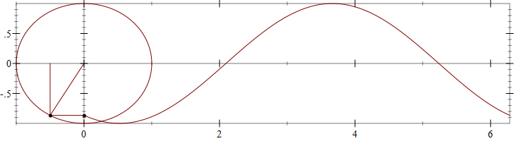
Plots are generated using the plot function, which creates the plot image from a list of “renderers”, each renderer representing one element of the plot. The animated plot will need to be drawn at various angles as the “dot” travels around the unit circle, so it is a good idea to separate the angle a from the rest of the plot, even if it is a constant in this example. Here is an explanation of each renderer used in the image above:
(axes)will draw the X, Y plot axes which intersect at origin(polar (lambda (theta) 1))will draw the unit circle at origin — thepolarrenderer will plot in polar coordinates, taking a function which converts an angle (theta) into a distance from origin, for a circle, this is simply 1.- the next three
linesrenderers will draw the radius at the current angle,a, and the projections onto the X and Y axes. polar-labelwill place a label in polar coordinates on the unit circle at the anglea— the renderer will draw a dot by default plus a text value. Since we are using an empty string for the label, only the dot will be visible, marking the position on the unit circle.point-labelwill place a label at a specified position — this time on the Y axis, just as withpolar-label, we use an empty label, so only a dot will be displayed.(function (lambda (x) (sin (+ a x))) 0 (* 2 pi))will draw the sine function. Thefunctionrenderer will plot the supplied function between two values (0 and 2Π in our case), and the argument to the sine function is offset by the angleato make sure the sine function has the same value at origin as the projection from the unit circle
If you are not familiar with the plot package, it would be a good idea to experiment with changing the angle a to various values and re-plot the image to see how the plot changes with the angle. You can also experiment with commenting out different renderers are and see what their contribution is to the overall plot.
The previous plot uses the same color and line widths for all plot elements, making it difficult to tell them apart. However, each renderer has keyword arguments which control the drawing parameters, such as colors and line widths. The documentation for the renderers shows the full list, but these are the most common arguments:
#:colordetermines the color of the renderer. This can be a RGB triplet, but it can also be a string, naming a color from the color database#:styledetermines the line style, such as dashed, solid, or even transparent#:widthspecifies the width of the line#:point-sizeand#:point-colorrepresent the size and color of the dots for labels.
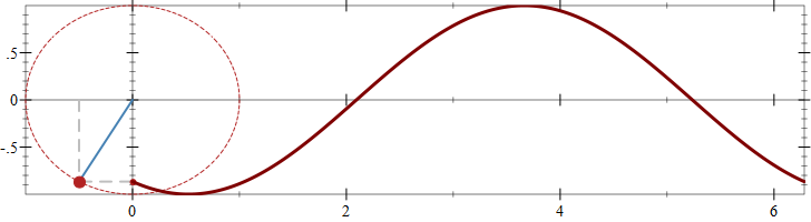
This is the same plot call, but this time each renderer has been styled to use different color, sizes and line styles:
1 2 3 4 5 6 7 8 9 10 11 12 13 14 15 16 |
#lang racket (require plot) (define a (* 10 (/ pi 3))) ; angle at which we draw the line and sine function (plot (list (axes) (polar (lambda (theta) 1) #:color "firebrick" #:style 'short-dash) (lines (list (vector 0 (sin a)) (vector (cos a) (sin a))) #:style 'long-dash #:color "gray" #:width 2) (lines (list (vector (cos a) 0) (vector (cos a) (sin a))) #:style 'long-dash #:color "gray" #:width 2) (lines (list (vector 0 0) (vector (cos a) (sin a)))#:color "steelblue" #:width 2) (polar-label (lambda (theta) 1) a "" #:point-size 10 #:point-color "firebrick") (point-label (vector 0 (sin a)) "" #:point-size 5 #:point-color "firebrick") (function (lambda (x) (sin (+ a x))) 0 (* 2 pi) #:width 3)) #:height (exact-round (* 100 2)) #:width (exact-round (* 100 (+ 1 (* 2 pi))))) |
There are several ways to generate plot animations, for example, you can generate individual images for each angle value a, save them to a file and use external tools to create a “movie”. Racket even has a library for writing animated GIF files. Here we’ll focus on writing plot animations which can be embedded in GUI applications.
The call to plot (and plot-snip) produces a snip% object, which is an interactive object that knows how to display itself and interact with the mouse — DrRacket REPL recognizes these objects and draws them in the REPL. The snip returned by the plot functions is a [2d-plot-snip%][2d-plot-snip] which provides two extra methods: set-mouse-event-callback and set-overlay-renderers. Together these methods can be used to implement interactive plots, but they can also be used separately.
The set-overlay-renderers method can be used to add new renderers to an existing plot and this can be used to implement animations: we can create a plot containing the “fixed” parts such as the axes and the unit circle and use set-overlay-renderers to construct the remaining elements periodically as the angle a increases:
Unfortunately, manipulating snips this way cannot be done when the snips are displayed in the REPL. This is because the REPL itself will create a copy of the snip and display the copy. The user program has no access to this copy so it cannot update it. However, we can add snips to GUI applications using the plot-container package and this will allow us to keep a reference to the plot snip and update it as needed. plot-container is not part of the standard Racket installation and will need to be installed using a raco command: raco pkg install plot-container.
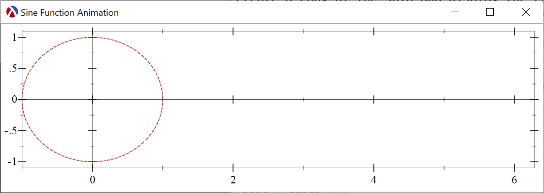
Here is a simple GUI application with a single toplevel window that shows the plot snip. The program still has access to the plot snip itself as the snip global variable:
1 2 3 4 5 6 7 8 9 10 11 12 13 14 15 16 17 |
#lang racket/gui (require plot plot-container) (plot-x-label #f) (plot-y-label #f) (define toplevel (new frame% [label "Sine Function Animation"] [height (exact-round (* 100 2.6))] [width (exact-round (* 100 (+ 1 (* 2 pi))))])) (define container (new plot-container% [parent toplevel])) (define snip (plot-snip (list (axes) (polar (lambda (theta) 1) #:color "firebrick" #:style 'short-dash)) #:x-min -1 #:x-max (* 2 pi) #:y-min -1.1 #:y-max 1.1)) (send container set-snip snip) (send toplevel show #t) |
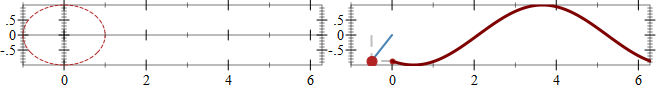
Running this program will create the empty looking plot in a separate window:
The actual renderers for the sine function can be produced by a separate function, which takes an angle as a parameter and returns the renderers. Note that this function does not call any of the plot functions but simply returns these renderers, these renderers can be passed to set-overlay-renderers to update the plot:
1 2 3 4 5 6 7 8 9 10 11 12 13 |
(define origin (vector 0 0)) (define (make-sine-renderers a) (define sin-a (sin a)) (define cos-a (cos a)) (define point-on-circle (vector cos-a sin-a)) (list (lines (list (vector 0 sin-a) point-on-circle) #:style 'short-dash #:color "gray" #:width 2) (lines (list (vector cos-a 0) point-on-circle) #:style 'short-dash #:color "gray" #:width 2) (lines (list origin point-on-circle) #:color "steelblue" #:width 2) (polar-label (lambda (theta) 1) a "" #:point-size 10 #:point-color "firebrick") (point-label (vector 0 sin-a) "" #:point-size 5 #:point-color "firebrick") (function (lambda (x) (sin (- a x))) 0 (* 2 pi) #:width 3))) |
In the DrRacket REPL we can call set-overlay-renderers with different arguments to make-sine-renderers to see how it all fits together, for example:
1 |
(send snip set-overlay-renderers (make-sine-renderers 1)) |
What remains is to create a function which produces sine function renderers at regular intervals and passes them to the plot snip for rendering. This can be a simple loop with a sleep call, but this will not produce good results for two reasons: first, the canvas redraw time cannot be controlled, so a call to set-overlay-renderers will simply queue a redraw request which will happen later and second, the mechanism we chose will produce a lot of garbage: each time we call make-sine-renderers the function will allocate data for the renderers, these will be displayed once, than never used again — as memory accumulates, Racket will stop the running program to reclaim the memory.
We cannot perfectly address these issue, but we can alleviate it: we’ll keep track of the animation time and run the garbage collector at regular intervals, hoping that its impact on performance will be smaller.
Instead of animating based on angle, we will animate based on time and we’ll use an angular velocity to calculate the angle corresponding to a timestamp: make-animation-frame produces the renderers at a time t and it does so simply by calculating the angle and calling make-sine-renderers:
The do-animation function is responsible for keeping track of the animation time, periodically calling make-animation-frame and updating the plot snip with the new renderers followed by a minor garbage collection. To ensure that each frame starts at a reasonably precise interval, the function keeps track of the duration of the redraw and garbage collection which is subtracted from the amount of time the function sleeps before starting a new iteration:
1 2 3 4 5 6 7 8 9 |
(define (do-animation fn #:frame-rate [frame-rate 60]) (define frame-time (/ 1 frame-rate)) (define start-timestamp (current-inexact-milliseconds)) (let loop ([timestamp (current-inexact-milliseconds)]) (send snip set-overlay-renderers (fn (/ (- timestamp start-timestamp) 1000.0))) (collect-garbage 'incremental) (define remaining (- frame-time (- (current-inexact-milliseconds) timestamp))) (sleep/yield (max 0 remaining)) (loop (current-inexact-milliseconds)))) |
Calling (do-animation make-animation-frame) produces a smooth looking animation:
Originally, set-overlay-renderers was indented to be used to add plot annotations, such as hover labels, in response to mouse events, however, the method can be used separately. Since, the “fixed” plot part will be rendered to a bitmap only once, and only the additional renderers will have to be recalculated and plotted, this can be more efficient than creating animations which render the entire plot area every frame.