Rendering the World Map Using the Racket Plot Package

2020-10-10 :: racket, data visualization

As part of writing the geoid package, I needed to visualize some geographic projections and I discovered that the 3D plotting facilities in the racket plot package can be easily used for this task. The geoid package and the projection it uses is somewhat complex, so, to keep things simple, this blog post covers the display of the country outlines on a globe loading the data from the GeoJSON file and using only basic plotting facilities.

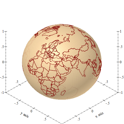
The image below is rendered entirely using the racket plot package, and it only takes a few lines a Racket code to load the data from a GeoJSON file and display it. You’ll only need a standard Racket installation, with no additional packages, but it does require some creative use of the 3D plot features.

Latitude, Longitude and the Unit Vector

The geographic data that define the outline of continents and countries uses latitude/longitude coordinates, but the racket graph plotting package does not directly understand these coordinates, so we’ll need to decide how to represent the data in a way that it can be plotted.

To keep things simple, we’ll approximate the Earth using a sphere of radius of 1, since the plot package does not really care what the radius of Earth is. The lat-lng->unit-vector function will convert a latitude/longitude coordinate into a 3D point on the unit sphere representing the earth, it is simply a wrapper around the 3d-polar->3d-cartesian function from the plot/utils package, since that function works with radians, and geographic coordinates are supplied in degrees:

(require plot plot/utils)

(define (lat-lng->unit-vector lat lng)
 (3d-polar->3d-cartesian 
   (degrees->radians lng)
   (degrees->radians lat)
   1))

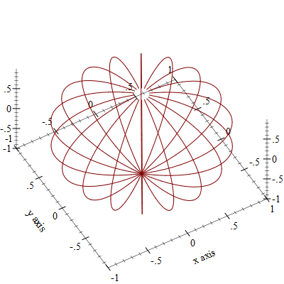
To verify that the function works as expected, we can try plotting some shape that is easy to recognize and see if they look correct. I choose to plot meridians, which are arcs on the sphere for the same longitude. The meridian function constructs a list of 3d points with a constant longitude, and constructs a lines3d renderer from these points:

(define (meridian lng)
  (define points
    (for/list ([lat (in-range -90.0 90.0 5.0)])
      (lat-lng->unit-vector lat lng)))
  (lines3d points))

A renderer produced by meridian can be passed to plot3d to be displayed, but we can also construct a list of these meridians to circle the entire sphere. The plot3d function can plot a list of renderers:

1 2	(plot3d (for/list ([lng (in-range -180 180 20)]) (meridian lng)))

If you type the above command in the DrRacket repl, the resulting plot can be rotated using the mouse, but here is an image of what it looks like:

The meridian lines in the previous plot make the outline of a sphere, but this might be difficult to see, since the plot package will not apply shading to the 3d lines and this reduces the depth perception. To help with that, we can add an actual sphere to the plot, which can be rendered using the polar3d renderer, specifying a function which simply returns 1 (the radius of the sphere), and also adds a color and some transparency to it:

(define unit-sphere
  (polar3d (λ (θ ϕ) 1.0)
           #:color "navajowhite"
           #:line-style 'transparent
           #:alpha 0.9))

The unit sphere can be added to the list of renderers for plotting, making the resulting plot easier to interpret. And, of course, running the code in DrRacket allows rotating the plot with the mouse:

1
2
3

(plot3d (cons unit-sphere 
              (for/list ([lng (in-range -180 180 20)])
                (meridian lng))))

Obtaining the World Map Data

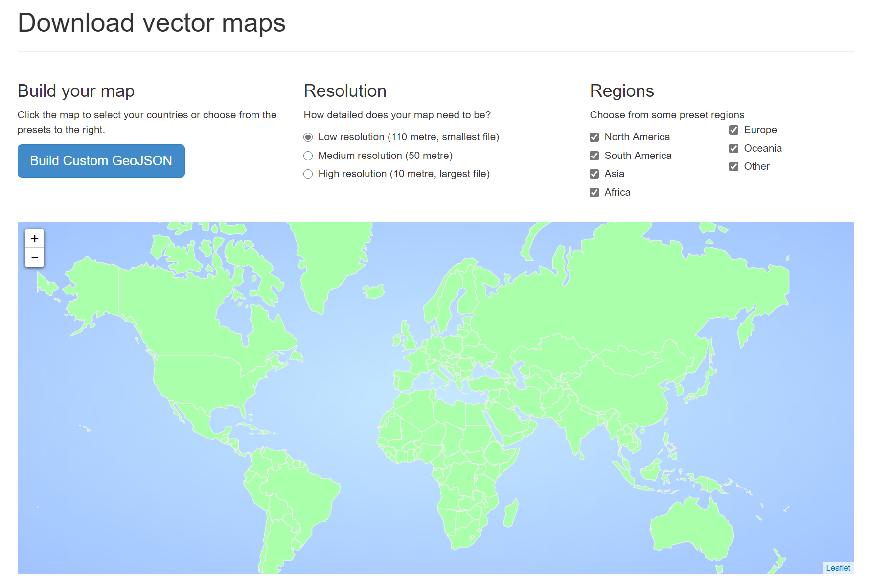
To create the world map, we’ll need the data containing the outlines of countries. After quick search, I discovered a website which allows downloading vector maps as GeoJSON files. The site is called https://geojson-maps.ash.ms/ , and the source for it is also available on GitHub. I simply selected all the available regions and downloaded a single GeoJSON file with the entire world map data.

Once downloaded from the website, the data can be loaded using the Racket json library:

1 2	(require json) (define world-data (call-with-input-file "./custom.geo.json" read-json))

The data file, even at 600kb in size is to large to understand it just by opening it in a text editor or printing it in the DrRacket REPL. In another blog post I showed how to load and inspect a large GeoJSON file by using a random sample of its contents, in this blog post, I’ll just summarize the structure of the file. The JSON file also contains some other geographic information, which we don’t use and will not be explained here.

the GeoJSON object is represented using normal Racket hash and list data structures, so the normal racket functions can be used to inspect and traverse it
all GeoJSON objects have a type key describing their type
the toplevel object is a “FeatureCollection” with the features key mapping to a list of GeoJSON objects, each feature defines a country outline..
each feature has a type of “Feature”, and a geometry gey defining the boundary of the country.
The geometry of each country is a “Polygon” containing a list of GPS points defining the contour the zone. Sometimes a time zone is defined by multiple contours, and this is shown by a “MultiPolygon” geometry type.

Plotting the World Map

To render the world data, we will need to traverse the world map data in the GeoJSON file and construct lines3d renderers for each of the polygons in this data set. Since the plot package can plot multiple such renderers, it is easier to have a separate renderer for each polygon, rather than using a single 3d line for the entire data set.

The make-renderers function will traverse each of the feature in the GeoJSON file, and construct a renderer for each of the Polygon or MultiPolygon construct inside it. It is a simple traversal of the nested hash and list structure of the object. The actual renderer is created by calling make-polygon-renderer, which is explained below.

(define (make-renderers world-map-data)
  (for/fold
      ([renderers '()])
      ([feature  (in-list (hash-ref world-map-data 'features))])
    (let* ([geometry (hash-ref feature 'geometry (lambda () (hash)))]
           [data (hash-ref geometry 'coordinates (lambda () null))])
      (case (hash-ref geometry 'type #f)
        (("Polygon") (cons (make-polygon-renderer data) renderers))
        (("MultiPolygon") (cons (for/list ([polygon (in-list data)])
                                  (make-polygon-renderer polygon))
                                renderers))
        (else (printf "Skipping ~a geometry" (hash-ref geometry 'type #f))
              renderers)))))

Finally, the make-polygon-renderer function will construct a lines3d from a single polygon. What GeoJSON calls a “polygon” it is actually a collection of polygons, the first one is an outline of the area (such as the country boundary in our case), while the remaining polygons represent the “holes” in the first area. To keep things simple, make-polygon-renderer constructs a lines3d renderer for each of these polygons:

(define (make-polygon-renderer polygons)
  (for/fold ([renderers '()])
            ([polygon (in-list polygons)] #:unless (null? polygon))
    (define points
      (for/list ([point (in-sequences
                         (in-list polygon)
                         (in-value (car polygon)))])
        (match-define (list lng lat _ ...) point)
        (lat-lng->unit-vector lat lng)))
    (cons (lines3d points) renderers)))

And that’s all it takes to create the plot: start with the unit sphere and add the line renderers on top:

1	(plot3d (list unit-sphere (make-renderers world-data)))

Final Thoughts

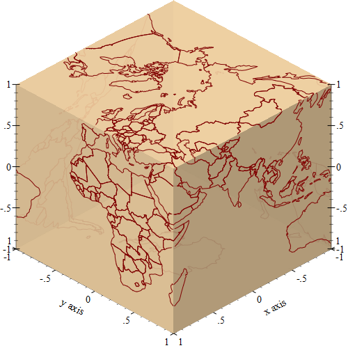
It might seem just a curiosity that the racket plot package can create these types of plots, however, I came across this functionality while trying to validate a package I wrote, which projects GPS coordinates onto the faces of a cube. While it is important to write tests to validate the behavior, it is also nice to be able to visualize the result. In this particular case, I build a plot which displays the projection, so I can validate it visually. The plot uses the same techniques as described in this blog post, but it uses the internals of the geoid library to provide the projection: