Timezone Visualization
The timezone-boundary-builder project publishes GeoJSON files with timezone boundaries based on OpenStreetMap data, and I though it would be an interesting project to load this data in Racket, build some map visualizations with it and explore some of the Racket drawing facilities.
The GeoJSON files can be downloaded from the releases section section of the timezone-boundary-builder project. There are two sets of files: one contains timezone data for the oceans and one only contains timezone data for the countries. In the examples below, I used the country data only, as this produces nicer maps. Besides, on the oceans, the timezones match the longitude boundaries of the globe.
Loading and inspecting the GeoJSON file
The GeoJSON timezone data can be loaded into Racket using read-json, and it takes about 25 seconds to load the 127Mb JSON file when using Racket 7.3 — this actually is a huge improvement over the previous Racket version which needed about 130 seconds to load the same file.
1 2 3 |
#lang racket (require json) (define timezone-data (call-with-input-file "./combined.json" read-json)) |
The JSON object is represented in Racket as a hash table for the key/value mappings and as a list for the arrays and this means that the object could be printed directly in the Racket REPL. However, this is a large object containing a lot of data so printing it will take a lot of time and, with a lot of data points printed, it will be difficult to see its structure. It is helpful to write a function to simplify the JSON object, discarding most of the data, so only a subset is shown — this will not be useful for processing the actual data, but it will help with having a smaller data structure on which to test the processing functions defined later. The function random-sample defined below does this: it creates a copy of its input object, but only keeps max-size items from the sublists inside the object:
1 2 3 4 5 6 7 8 9 10 11 12 13 14 15 16 |
(define (random-sample object [max-size 5]) (cond ((hash? object) (for/hash ([(k v) (in-hash object)]) (values k (random-sample v max-size)))) ((list? object) (let ([len (length object)]) (if (> len max-size) (let ([samples (sort (build-list max-size (lambda (x) (random len))) <)]) (for/list ([(x position) (in-indexed (in-list object))] #:when (member position samples)) (random-sample x max-size))) (for/list ([x (in-list object)]) (random-sample x max-size))))) (#t object))) |
Running the code on the timezone data produces the output below, which is easier to follow when trying to write data manipulation functions for the timezone data:
1 2 3 4 5 6 7 8 9 10 11 12 13 14 15 16 17 18 |
> (random-sample timezone-data 2) '#hash((features . (#hash((geometry . #hash((coordinates . (((31.5209 -27.31543) (30.91294 -26.86306)))) (type . "Polygon"))) (properties . #hash((tzid . "Africa/Mbabane"))) (type . "Feature")) #hash((geometry . #hash((coordinates . ((((72.452033 -5.430984) (71.531301 -5.286587))) (((72.531264 -7.062455) (72.153049 -7.249701))))) (type . "MultiPolygon"))) (properties . #hash((tzid . "Indian/Chagos"))) (type . "Feature")))) (type . "FeatureCollection")) > |
The json-write function can be used to write out the result in JSON format, and this can be used to generate smaller subsets of the data, after all, it takes about half a minute to load the actual data, which can be too much when the program is evaluated repeatedly during development.
1 2 3 4 5 6 7 8 9 10 11 12 13 14 15 16 17 18 19 20 21 22 23 24 25 26 |
{ "type":"FeatureCollection", "features":[ { "type":"Feature", "geometry": { "type":"Polygon", "coordinates":[[[31.5209,-27.31543],[30.91294,-26.86306]]] }, "properties": { "tzid":"Africa/Mbabane" } }, { "type":"Feature", "geometry": { "type":"MultiPolygon", "coordinates":[[[[72.452033,-5.430984],[71.531301,-5.286587]]], [[[72.531264,-7.062455],[72.153049,-7.249701]]]] }, "properties": { "tzid":"Indian/Chagos" } } ] } |
With the simplified version, it is easy to follow the structure of the JSON file. The Wikipedia GeoJSON article explains the overall structure of a GeoJSON document, but here is a summary:
- all GeoJSON objects have a
typekey describing their type - the toplevel object is a “FeatureCollection” with the
featureskey mapping to a list of GeoJSON objects, each feature defining a time zone boundary. - each feature has a
typeof “Feature”, ageometrydefining the boundary of the timezone and apropertieskey which contains the timezone name in thetzidproperty. The name of the timezones are the same as the IANA Timezones. - The geometry of each time zone is a list of GPS points defining the contour the zone. Sometimes a time zone is defined by multiple contours, and this is shown by a “MultiPolygon” geometry type.
Since Racket represents a JSON object using hash tables and lists, it is easy to write functions which manipulate the data. For example, to find out how many timezones there are, we can count the number of features in the object:
As an exercise, I wrote some functions to count the number of points in the database as well as in all the timezones. The program is available in this github gist (the “example0.rkt” file), and here is a summary of its findings: there are 426 timezones and all of them are defined using 5′728′474 GPS points. Here is a list of the timezones defined by the largest number of points — the number of points does not seem to correlate with the actual size of the timezone:
| TimeZone | Point Count | TimeZone | PointCount |
| Europe/Berlin | 142′178 | Asia/Shanghai | 123′836 |
| America/Santiago | 118′996 | Europe/Vienna | 110′643 |
| Asia/Kolkata | 94′538 | Europe/Prague | 92′587 |
| Europe/Moscow | 90′441 | Asia/Karachi | 75′744 |
| Asia/Krasnoyarsk | 73′401 | Asia/Bangkok | 73′017 |
| Asia/Yakutsk | 70′839 | Asia/Vladivostok | 70′588 |
| Africa/Johannesburg | 61′474 | Asia/Yekaterinburg | 57′482 |
| Asia/Tehran | 56′481 | Europe/Paris | 56′370 |
| Africa/Lubumbashi | 55′929 | Asia/Irkutsk | 54′693 |
| Europe/Rome | 54′293 | Asia/Urumqi | 52′500 |
Drawing the timezone boundaries as a map
The best way to look at GeoJSON data is to draw it on a map, so in the next section we’ll explore how to draw these timezones using Racket and will produce the picture shown at the top of the blog post. However, this task requires some more advanced use of Racket’s drawing capabilities and before we can look at it, it is worth refreshing some of the more important concepts.
Racket Drawing Toolkit Refresher
Drawing Contexts
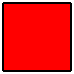
Drawing in Racket is done using a drawing context, which is an abstract interface for drawing commands. A drawing context can be created for a canvas% for drawing in a GUI application or a bitmap for drawing on a bitmap, and, regardless of where the drawing will be displayed, the drawing commands are the same. Here is an example on how to create a bitmap containing a red rectangle:
1 2 3 4 5 6 7 8 9 |
#lang racket (require racket/draw) (define dc (new bitmap-dc% [bitmap (make-object bitmap% 250 250)])) (send* dc (set-pen (send the-pen-list find-or-create-pen "black" 5.0 'solid)) (set-brush (send the-brush-list find-or-create-brush "red" 'solid)) (draw-rectangle 10 10 (- 250 20) (- 250 20))) (define bm (send dc get-bitmap)) (send bm save-file "example1.png" 'png) |
In the example above, the bitmap-dc% is a concrete device context implementing the dc<%> interface and drawing onto a bitmap and once created it is sent three commands: set-pen, set-brush and draw-rectangle. The drawing commands, such as draw-rectangle will use the currently set pen for the outline of the drawing and the currently set brush for the “fill”. Pen and Brush objects use up drawing resources and to avoid unnecessary creation of identical pen and brushes, the-pen-list and the-brush-list databases can be used: they will create a new resource if needed, but otherwise just return a previously created one. Finally, a bitmap object can be saved into a file using save-file. The result is not very exciting yet:
Context Scale and Offset
By default, a device context has the origin (0, 0) in the top left corner and its size is the same as the underlying target bitmap or canvas. Drawing commands must take these into account if they want to draw things relative to some anchor points: for example, to draw a vertical line in the middle of the device context, its size must be retrieved, and the middle point calculated, as it will be different depending on the size of the canvas. An alternative is to change the coordinate system and scale of the device context to known values, so that drawing commands are always done in known coordinates. In the example below, the origin of the device context is moved to its middle and the device is scaled such that the device context coordinates are always between –1 and 1. With this setup, the drawing commands are now independent of the size of the bitmap, and drawing a vertical line in the middle is always done using draw-line 0 -1 0 1:
1 2 3 4 5 6 7 8 9 10 11 12 13 14 |
#lang racket (require racket/draw) (define dc (new bitmap-dc% [bitmap (make-object bitmap% 250 250)])) (send* dc (set-origin 250/2 250/2) (set-scale 250/2 250/2) (set-pen (send the-pen-list find-or-create-pen "black" 0.00001 'solid)) (set-brush (send the-brush-list find-or-create-brush "black" 'transparent)) (draw-rectangle -1 -1 2 2) (set-brush (send the-brush-list find-or-create-brush "red" 'solid)) (draw-line -1 0 1 0) (draw-line 0 -1 0 1)) (define bm (send dc get-bitmap)) (send bm save-file "example2.png" 'png) |

DC paths
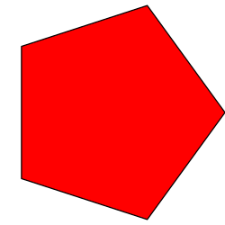
The device context interface provides primitives for drawing basic shapes, such as lines, rectangles and ellipses, but for more complex shapes, a dc-path% can be used, this is an object holding a set of lines and curves. A dc-path% can be open or closed, and a closed dc path will have its interior filled with the current brush color. Below is an example of drawing a pentagon using a dc-path%, since we use device scaling, the points for the shape can be defined on the unit circle:
1 2 3 4 5 6 7 8 9 10 11 12 13 14 15 16 17 18 19 20 21 |
#lang racket (require racket/draw) (define path (new dc-path%)) (send path move-to 1 0) (for ([p (in-range 0 (* 2 pi) (/ (* 2 pi) 5))]) (define x (cos p)) (define y (sin p)) (send path line-to x y)) (send path close) (define dc (new bitmap-dc% [bitmap (make-object bitmap% 250 250)])) (send* dc (set-smoothing 'smoothed) (set-scale 250/2 250/2) (set-origin 250/2 250/2) (set-pen (send the-pen-list find-or-create-pen "black" 0.01 'solid)) (set-brush (send the-brush-list find-or-create-brush "red" 'solid)) (draw-path path)) (define bm (send dc get-bitmap)) (send bm save-file "example3.png" 'png) |
Drawing the timezone map
The overall process for drawing the timezones is straightforward: for each time zone (which is a feature in the GeoJSON file), construct a dc-path% with all the points that are part of its definition, than render the path using a distinct color. There are, however, a few details to discuss.
The toplevel function for drawing the bitmap takes as parameters the timezone GeoJSON data and the width and height of the desired bitmap. It sets up a bitmap device context, and sets its scale such that the entire drawing area is from 0 to 1, it than iterates over the features in the GeoJSON file (each feature is a timezone shape definition), it assigns a brush color for filling in the area, than calls draw-feature to draw the actual timezone shape.
1 2 3 4 5 6 7 8 9 10 11 12 |
(define (make-timezone-bitmap tzdata width height) (define dc (new bitmap-dc% [bitmap (make-object bitmap% width height)])) (send* dc (set-scale width height) (set-smoothing 'smoothed) (set-pen (send the-pen-list find-or-create-pen "black" (* 0.5 (/ 1 width)) 'solid))) ;; Iterate over each feature (timezone) and render it (for ([feature (in-list (hash-ref tzdata 'features))] [color (in-cycle (in-list color-map))]) (send dc set-brush (send the-brush-list find-or-create-brush color 'solid)) (draw-feature dc feature)) (send dc get-bitmap)) |
Ideally, we would like to render each time zone in a distinct color, but for now, the code just cycles through a palette of colors, which means that some timezones will share the same color. For completeness, here is the color table, which is a list of color% objects:
1 2 3 4 5 6 7 8 9 10 11 |
(define color-map (list (make-object color% 78 121 165) (make-object color% 241 143 59) (make-object color% 224 88 91) (make-object color% 119 183 178) (make-object color% 90 161 85) (make-object color% 237 201 88) (make-object color% 175 122 160) (make-object color% 254 158 168) (make-object color% 156 117 97) (make-object color% 186 176 172))) |
The draw-feature function will retrieve the coordinates for the timezone and call draw-polygon, or if the feature is a multi-polygon, it will call draw-polygon for each polygon in the timezone definition, since a timezone can be defined by multiple polygons.
1 2 3 4 5 6 7 |
(define (draw-feature dc feature) (let* ([geometry (hash-ref feature 'geometry (lambda () (hash)))] [data (hash-ref geometry 'coordinates (lambda () null))]) (case (hash-ref geometry 'type #f) (("Polygon") (draw-polygon dc data)) (("MultiPolygon") (for ([polygon (in-list data)]) (draw-polygon dc polygon))) (else (printf "Skipping ~a geometry" (hash-ref geometry 'type #f)))))) |
The draw-polygon function receives a polygon, which is a list of GPS coordinates, constructs a closed dc-path% from them and draws it onto the device context. A GeoJSON polygon is actually defined as a list of lists, the first list being the “outside” polygon, and the remaining one are the “holes” inside the main shape. The code below uses sub-paths of the main dc-path% to create these holes.
1 2 3 4 5 6 7 8 9 10 |
(define (draw-polygon dc polygons) (define path (for/fold ([path #f]) ([polygon (in-list polygons)] #:unless (null? polygon)) (define sub-path (new dc-path%)) (send/apply sub-path move-to (lat-lon->map-point (car polygon))) (for ([point (in-list (cdr polygon))]) (send/apply sub-path line-to (lat-lon->map-point point))) (send sub-path close) (if path (begin (send path append sub-path) path) sub-path))) (and path (send dc draw-path path 0 0))) |
Finally, the lat-lon->map-point function takes a pair of GPS coordinates (latitude, longitude) and converts them into normalized coordinates which are values between 0 and 1, where 0 and 1 are the edges of the map. The projection we use here is Mercator, which is what is used by most maps, but any projection would be adequate for the task. Note that the device context scale shows its usefulness here: since the device is scaled, the normalized coordinates can be drawn directly onto the device context, without having to worry about adjusting them. Also, changing the rest of the code does not need to worry about changing the size of the bitmap.
1 2 3 4 5 |
(define (lat-lon->map-point coordinates) (match-define (list lon lat _ ...) coordinates) (define-values (x y) (values (degrees->radians lon) (asinh (tan (degrees->radians lat))))) (list (/ (+ 1 (/ x pi)) 2) (/ (- 1 (/ y pi)) 2))) |
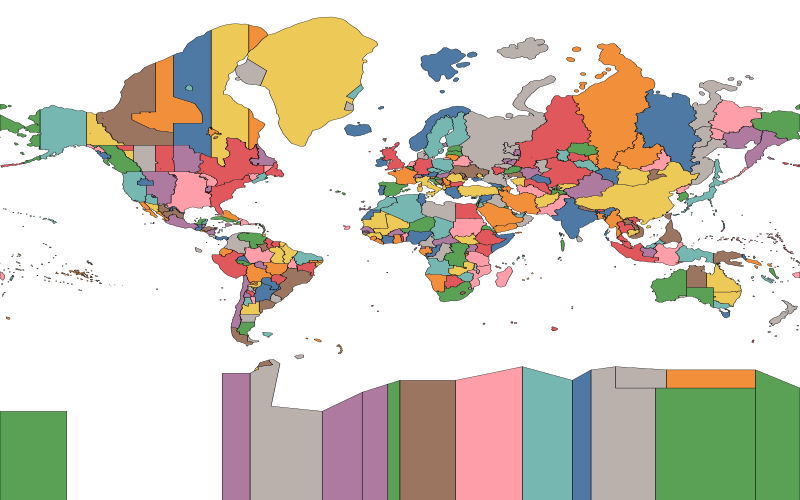
You can find the entire program as a github gist (the "example4.rkt file), and the output is shown below. The entire program is less than 100 lines long and only uses standard Racket libraries and no external packages.
1 2 3 |
(define timezone-data (call-with-input-file "./combined.json" read-json)) (define bm (make-timezone-bitmap timezone-data 800 500)) (send bm save-file "timezone-map.png" 'png 100 #:unscaled? #t) |
The final result is shown below, but the map requires some explanations. First, the Mercator projection used for the map does not work very well at high latitudes and breaks down at extreme ones, so Antarctica looks unfamiliar, this is not helped by the fact that parts of Antarctica are not covered by any timezones. Second, the white area of the map represents oceans, where no specific timezones are defined — in these area, the timezone can be directly determined from the longitude — the timezone-boundary-builder project also provides GeoJSON files with timezones for the ocean areas. Finally, these are timezone boundaries, not country boundaries, and, while some countries can be recognizable, other are not.
Unique timezone colors
The code above cycled through a color map containing only 10 unique colors. While it produced a pleasing result, many timezones share the same colors, including sometimes neighboring colors. While 4 colors are sufficient to color any map, such that no adjacent regions have the same color, it is much simpler to just assign a unique color to each time zone.
The idea behind this is to allocate a unique ID to each time zone, than allocate colors for each of these IDs. The tzdata structure keeps information about a time zone, its ID and color. The allocate-tzdata will create a list of tzdata structures, assign an unique ID by incrementing a counter and creating a color% object for it:
1 2 3 4 5 6 7 8 9 10 |
(struct tzdata (name id color) #:transparent) (define (allocate-tzdata node) (define next-id 1) ; start at 1, 0 is reserved for "no tz data", the oceans (for/list ([tznode (in-list (hash-ref node 'features))]) (define name (tz-name tznode)) (define id next-id) (set! next-id (add1 next-id)) (define color (allocate-color id)) (tzdata name id color))) |
There are multiple ways to generate colors from integer identifiers, but the simplest method is to treat each digit in the number as one of the R, G, B channels, since there are 426 time zones, this seems sufficient. In addition to that, to separate the colors a bit more, each digit in the channel will be multiplied by 28, so each color channel is used evenly. I.e, rather than using 0, 1, … 9 for the red channel, we’ll use 0 * 28, 1 * 28, … 9 * 28 for these values, and since 9 * 28 is 252, all values will be below the maximum 255 value:
1 2 3 4 5 |
(define (allocate-color id) (let* ((b (exact-floor (/ id 100))) (g (exact-floor (/ (- id (* b 100)) 10))) (r (exact-floor (- id (* b 100) (* g 10))))) (make-object color% (* r 28) (* g 28) (* b 28)))) |
By the way, the tz-name is just a helper function which retrieves the tzid property of a timezone GeoJSON feature:
Finally, the make-timezone-bitmap toplevel function will need to be updated to allocate colors for the timezones and use them for rendering:
1 2 3 4 5 6 7 8 9 10 11 12 13 |
(define (make-timezone-bitmap tzdata width height) (define tz-data (allocate-tzdata timezone-data)) (define dc (new bitmap-dc% [bitmap (make-object bitmap% width height)])) (send* dc (set-scale width height) (set-smoothing 'smoothed) (set-pen (send the-pen-list find-or-create-pen "black" (* 0.5 (/ 1 width)) 'solid))) ;; Iterate over each feature (timezone) and render it (for ([feature (in-list (hash-ref tzdata 'features))]) (define color (time-zone-color tz-data (tz-name feature))) (send dc set-brush (send the-brush-list find-or-create-brush color 'solid)) (draw-feature dc feature)) (send dc get-bitmap)) |
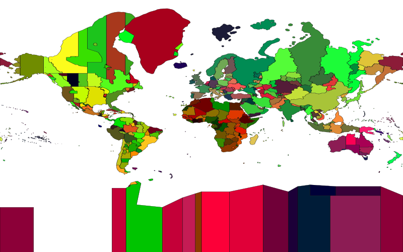
The result is shown below. The code does not make use of all colors, since it only uses about half of the colors that could be allocated using our strategy:
Rendering a subset of the map
The set-origin and set-scale methods of a device context can be used to render a subset of the map, without having to change the rest of the rendering code. To render the map between two GPS coordinates, min-coord and max-coord, we’ll first have to convert them into normalized coordinates (between 0 and 1) using lat-lon->map-point, than calculate scaling values such that the X and Y coordinates between the two points correspond to the actual width and height of the bitmap. The origin will have to be translated such that the point at min-coord is at (0,0) — this has to be a negative adjustment. The setup-dc function below does all this, preparing a device context to render a subset of the map between two GPS locations:
1 2 3 4 5 6 7 8 9 10 11 12 |
(define (setup-dc dc min-coord max-coord) (define-values (width height) (send dc get-size)) (match-define (list xmin ymin) (lat-lon->map-point min-coord)) (match-define (list xmax ymax) (lat-lon->map-point max-coord)) (define-values (xscale yscale) (values (/ width (- xmax xmin)) (/ height (- ymax ymin)))) (define-values (xorigin yorigin) (values (- (* xmin xscale)) (- (* ymin yscale)))) (send* dc (set-origin xorigin yorigin) (set-scale xscale yscale) (set-smoothing 'smoothed) (set-pen (send the-pen-list find-or-create-pen "black" (* 0.5 (/ 1 xscale)) 'solid)))) |
The main rendering function, make-timezone-bitmap remains largely the same, except it now calls setup-dc to prepare the bitmap and the rest of the drawing functions remain completely unchanged, as the drawing code will keep track of the current target bitmap size an clipping regions:
1 2 3 4 5 6 7 8 9 10 |
(define (make-timezone-bitmap tzdata min-coord max-coord width height) (define dc (new bitmap-dc% [bitmap (make-object bitmap% width height)])) (setup-dc dc min-coord max-coord) ;; Iterate over each feature (timezone) and render it (for ([feature (in-list (hash-ref tzdata 'features))] [color (in-cycle color-map)]) (send dc set-brush (send the-brush-list find-or-create-brush color 'solid)) (draw-feature dc feature)) (send dc get-bitmap)) |
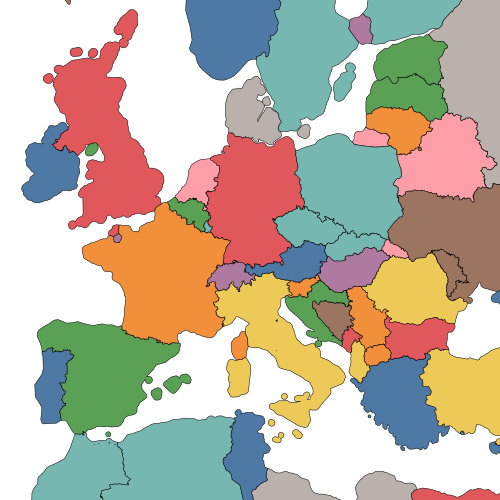
To test this code, I visited openstreetmap.org and obtained two GPS coordinates for the rough bounding box of Europe. To render the European timezones I used the following call:
Conclusions
The Racket program used to generate these maps has less than 100 lines of code and only uses features from a standard Racket installation, I suppose this is an example of what “batteries included” means.
I was also pleasantly surprised that the Racket drawing library can handle large drawing requests: some of the dc-path% objects have in excess of 100′000 lines and most of them have more than 50′000, with most of the lines being less than the pixel size of the resulting bitmap. Without any optimizations, the code above loads a huge JSON file and renders a map with a total of 5 million lines in just over a minute on my machine — when I started working on this code, I expected I will need to run some line simplification algorithms for the timezone boundaries, but this proved unnecessary. There are several optimizations that could be done to make the rendering faster, but since timezone boundaries change less often than the 1 – 2 minute rendering time, it is simpler to just keep the generated image around.
I uploaded all the programs used to generate the maps in this blog post to this GitHub Gist, you can run them directly and further experiment with them.