Timezone Lookup (an adventure in program optimization)
… in which we use GeoJSON data for timezone boundaries to determine the time zone for a given location, and learn a few things about the performance of Racket programs.
In my previous blog post I used geographic time zone boundaries from a GeoJSON file to create visual maps of these boundaries, but this data can also be used to determine the time zone for a certain location. In this blog post, we’ll implement a function which takes a GPS coordinate and returns the name of the time zone where this location. For the lookup itself, we’ll perform a point-in-polygon test on the polygons which define the time zones, determining which one contains the given coordinates. Since the time zone boundary definitions contain many thousands of points, with the top 20 timezones containing in excess of 50′000 points, we’ll need to be mindful of the performance of our lookup function.
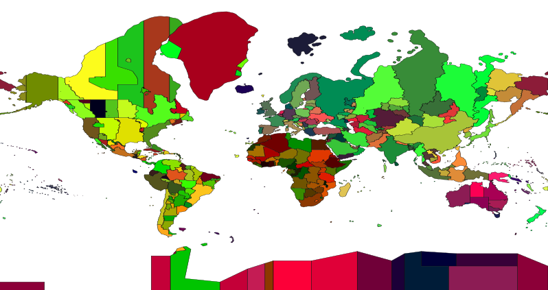
World Timezones
The first implementation uses the GeoJSON object directly and, while the implementation is straightforward and passes a comprehensive test suite, it is also very slow, taking about 8 seconds for one lookup. Since this implementation is too slow for anything except a proof-of-concept implementation, it is time to look into speeding things up. We’ll work on the improvements by running a profiler to measure running times for various functions and try to improve them.
The first improvement is to use bounding boxes to avoid an expensive point-in-polygon test when the point is well outside the polygon. This improvement brings down the running time of tz-lookup to about 80 milliseconds, making it 100 times faster than the initial version, and, for many practical purposes, making this function usable. Still, but we’ll continue exploring further improvements.
The next improvement is to convert the GeoJSON data into more specific structures and in particular to change the list of points representing the polygons into vectors. This improvement brings the tz-lookup time down to 36.9 milliseconds, which is a 54% improvement over the previous version. It looks like vectors are faster than lists even for sequential traversal, which is the strong point for lists.
The previous improvement forced us to do some memory allocations to convert points back to lists for passing around to other functions. Removing these unnecessary allocations gave us another 10% improvement, bringing the tz-lookup time down to 33.27 milliseconds.
We’ll try to use flvectors to store floating point values more efficiently and hope to make the program faster, but this is not the case, the program becomes 10% slower as a result. This shows the importance of measuring the execution time while attempting to optimize the code.
Finally, we’ll convert one of the functions, which uses a lot of floating point computations to use flonum operations, which the Racket compiler can optimize better (according to the documentation, anyway). This turns out to be true, and the execution time is improved by another 10%, recuperating the performance losses from the previous step.
Write the tests first
Before we start implementing the actual timezone lookup code, it is best to prepare a test suite, to ensure that the code works correctly. The workings of the test suite are pretty simple: just check that some GPS coordinates produce the correct timezone result, but which GPS coordinates should we use? Well, the tz-lookup project has a pretty comprehensive test suite, built, presumably, around a lot of tricky cases of GPS to timezone mappings. While our timezone lookup implementation will be quite different from that project, we can “borrow” their test cases.
We will structure the test data in a way that is convenient for Racket: as a list containing a latitude, longitude and corresponding timezone entry, and place them in a separate file with the following contents:
1 2 3 4 5 6 7 8 |
;; this is the tz-test-cases.rktd file ( ( 40.7092 -74.0151 "America/New_York") ( 42.3668 -71.0546 "America/New_York") ( 41.8976 -87.6205 "America/Chicago") ( 47.6897 -122.4023 "America/Los_Angeles") ;; ... more test cases here ) |
With the test data ready, we can write our test suite, which reads in the data from the file, and calls the tz-lookup function no the latitude,longitude pairs and checks the returned result against the correct one. Unsurprisingly, running the program below will fail all the test cases, as the tz-lookup simply returns #f for now:
1 2 3 4 5 6 7 8 9 10 11 12 |
#lang racket (define (tz-lookup lat lon) ;; does not do anything useful, will implement it later #f) (module+ test (require rackunit) (define test-data (call-with-input-file "./tz-test-cases.rktd" read)) (for ([test-case (in-list test-data)]) (match-define (list lat lon tzname) test-case) (check-equal? (tz-lookup lat lon) tzname))) |
The timezone lookup function implementation
The lookup function works by taking the latitude/longitude coordinates and checking if they are inside any of the time-zone definition polygons in the time zone GeoJSON data file published by the timezone-boundary-builder project. The Timezone Visualisation blog post contains some more detail about the structure of the data file, but here is a short overview:
- The GeoJSON is a FeatureCollection, containing a list of Features
- Each Feature represents a time zone, named by the
tzidproperty - Each Feature has a Geometry, which is either a Polygon or a MultiPolygon, which is just a collection of Polygons
- Each Polygon is defined as a list of points representing its outline and zero or more lists of points representing the “holes”.
First we define some functions to load the data and prepare the list of timezone features to check. These functions are trivial at this stage, but having defined allows us to measure the time it takes to load and prepare the data. We than define the global features variable to hold the list of features to check:
The tz-lookup function will traverse the list of features calculating how probable is that the point at lat/lon is inside each feature (this is the feature-winding-number function which we will discuss later), than filters out all features which have a low probability. Finally, if one candidate is found, it is returned, otherwise, a candidate is selected by the select-candidate function.
1 2 3 4 5 6 7 8 9 10 |
(define (tz-lookup lat lon) (define candidates (for/list ([feature (in-list features)]) (define wn (feature-winding-number feature lat lon)) (list (feature-name feature) wn))) ;; Keep only candidates that have a large winding number (define filtered (for/list ([c (in-list candidates)] #:unless (< (second c) 0.1)) c)) (cond ((null? filtered) #f) ((= (length filtered) 1) (first (first filtered))) (#t (select-candidate filtered)))) |
The feature-name is a simple convenience function which retrieves the tzid property from the GeoJSON node, this property holds the time zone name:
The select-candidate function is responsible for selecting a time zone when multiple options are available: time zones are defined by political boundaries and sometimes two countries make claim to the same territory. Our select-candidate function handles only one such case, the “Asia/Shanghai” vs “Asia/Urumqi”:
1 2 3 4 5 6 7 8 9 10 11 12 13 14 |
(define (select-candidate candidates) (define sorted (sort candidates > #:key second)) (match sorted ;; NOTE candidates are sorted by their winding number, W1 >= W2! ((list (list n1 w1) (list n2 w2) other ...) (if (> (- w1 w2) 1e-2) n1 ; w1 is definitely greater than w2 (cond ((or (and (equal? n1 "Asia/Shanghai") (equal? n2 "Asia/Urumqi")) (and (equal? n1 "Asia/Urumqi") (equal? n2 "Asia/Shanghai"))) "Asia/Urumqi") ; conflict zone (#t n1)))) ((list (list n1 w1) other ...) n1))) |
The check if a point is inside the polygon we’ll use the winding number algorithm as our point in polygon test. Before we do that, we have to descend though the GeoJSON nodes to get to the actual polygons. All the functions below, starting with feature-winding-number simply traverse the GeoJSON data:
1 2 3 4 5 6 7 8 9 10 11 12 13 14 15 16 17 18 19 20 21 22 23 24 25 26 |
(define (feature-winding-number feature lat lon) (for/fold ([wn 0]) ([shape (in-list (feature-shapes feature))]) (max wn (shape-winding-number shape lat lon)))) (define (feature-shapes feature) (let ([geometry (hash-ref feature 'geometry (lambda () (hash)))]) (let ([shapes (hash-ref geometry 'coordinates null)] [type (hash-ref geometry 'type #f)]) (cond ((equal? type "Polygon") (list shapes)) ((equal? type "MultiPolygon") ;; Must be in any of the shapes shapes) (#t (error (format "inside-feature? unsupported geometry type: ~a" type))))))) (define (shape-outline p) (first p)) (define (shape-holes p) (rest p)) (define (shape-winding-number p lat lon) (let ([outline (shape-outline p)] [holes (shape-holes p)]) (if (for/first ([h (in-list holes)] #:when (> (polygon-winding-number h lat lon) 0.9999)) #t) 0 (polygon-winding-number outline lat lon)))) |
The polygon-winding-number function is the one that does the actual work: it calculates the winding number of a polygon with respect the point at lat/lon. If this winding number is greater than 1, the point is inside the polygon, otherwise it is not. The function works, by iterating over each polygon segment, which are pairs of adjacent points, accumulating the subtended angle of the segment with respect to the lat/lon point. Special care is taken to close the polygon and calculate the angle of the last point to the first:
1 2 3 4 5 6 7 8 9 10 11 12 |
(define (polygon-winding-number poly lat lon) (define p0 (list lon lat)) (let loop ([winding-angle 0] [remaining-points poly]) (if (null? remaining-points) (abs (/ winding-angle (* 2 pi))) (let ([p1 (first remaining-points)] [p2 (if (null? (rest remaining-points)) (first poly) ; cycle back to beginning, closing the polygon (second remaining-points))]) (define angle (subtended-angle p0 p1 p2)) (loop (+ winding-angle angle) (rest remaining-points)))))) |
The subtended-angle requires some understanding of the dot product and cross product operations on vectors and it works as follows: the angle between the vectors p0->p1 and p0->p2 is calculated from the dot product of the two vectors and the sign is determined from the cross product of the same two vectors, the sign is needed to determine if the p1->p2 vector is traversed in clockwise or counter-clockwise direction. Too keep the code short, rather than defining vector operations for subtraction, length, dot-product and cross-product, all these are done in the function itself:
1 2 3 4 5 6 7 8 9 10 11 12 13 14 15 16 17 18 19 20 |
(define (subtended-angle p0 p1 p2) (match-define (list x0 y0) p0) (match-define (list x1 y1) p1) (match-define (list x2 y2) p2) (define s1x (- x1 x0)) (define s1y (- y1 y0)) (define s1len (sqrt (+ (* s1x s1x) (* s1y s1y)))) (define s2x (- x2 x0)) (define s2y (- y2 y0)) (define s2len (sqrt (+ (* s2x s2x) (* s2y s2y)))) (define dot-product (+ (* s1x s2x) (* s1y s2y))) (if (or (zero? dot-product) (zero? s1len) (zero? s1len)) 0 (let ([angle (acos (min 1.0 (/ dot-product (* s1len s2len))))]) (define cross-magnitude (- (* (- x1 x0) (- y2 y0)) (* (- y1 y0) (- x2 x0)))) (* angle (sgn cross-magnitude))))) |
If you are not familiar with vector algebra, the above explanations are not sufficient to understand how the winding number and the angle between vectors are calculated, and why the winding number is a good “point-in-polygon” test. I suggest you visit the linked Wikipedia pages for more information about these.
Does the code work? Yes it does! I was pleasantly surprised that it passes all the tests in the test suite, except for the maritime time zones which are not handled by our example. Unfortunately, the code runs very slowly: it took more than two hours on my machine to run the 996 time zone lookups from the test suite. Running the code through a profiler shows that the tz-lookup function takes between 6 and 15 seconds to run, with an average of about 8 seconds. While the implementation is good as a proof-of-concept, it needs some serious speed improvements before it can be used for practical purposes.
| function | total calls | total time (ms) | min (ms) | max (ms) | average (ms) |
| load-geojson | 1 | 13168.78 | 13168.78 | 13168.78 | 13168.78 |
| prepare-features | 1 | 0 | 0 | 0 | 0 |
| tz-lookup | 996 | 8288679.23 | 6984.56 | 15712.09 | 8321.97 |
| feature-winding-number | 424296 | 8287721.95 | 0 | 2754.98 | 19.53 |
| shape-winding-number | 1174284 | 8286076.95 | 0 | 2754.97 | 7.06 |
| polygon-winding-number | 1437228 | 8284665.13 | 0 | 2754.97 | 5.76 |
| subtended-angle | 5804339400 | 1747306.32 | 0 | 52.98 | 0.0003 |
Looking at the profiling results, we can see that the tz-lookup function takes on average about 8 seconds to run, however none of the functions it calls takes that long. The problem is not with the speed of polygon-winding-number itself, but with the number of times it is called: for each invocation of tz-lookup, there are about 1443 calls to polygon-winding-number, so our first focus needs to be to reduce the number of these calls.
Bounding Boxes
For most of the points that polygon-winding-number will have to check, the point will be well outside the polygon being tested, so, rather than going over all those points, we could calculate the Bounding Box of the polygon and only calculate the winding number if the point is within the bounding box.
Here are the definitions for he bbox structure, the inside-bbox? check and the make-bbox function which calculates the bounding box from a set of points:
1 2 3 4 5 6 7 8 9 10 11 12 13 14 15 16 17 18 19 |
(struct bbox (min-x min-y max-x max-y)) (define (inside-bbox? bb lat lon) (match-define (bbox min-x min-y max-x max-y) bb) (and (>= lon min-x) (<= lon max-x) (>= lat min-y) (<= lat max-y))) (define (make-bbox points) (if (null? points) #f (let ([p0 (first points)]) (let loop ([min-x (first p0)] [min-y (second p0)] [max-x (first p0)] [max-y (second p0)] [remaining (rest points)]) (if (null? remaining) (bbox min-x min-y max-x max-y) (let ([p1 (first remaining)]) (loop (min min-x (first p1)) (min min-y (second p1)) (max max-x (first p1)) (max max-y (second p1)) (rest remaining)))))))) |
We can than implement polygon-winding-number to check for the bounding box first, and only call the polygon-winding-number-internal function when the point is inside. The internal function contains the previous body of polygon-winding-number (unchanged) and will not be shown here:
This leaves us with the implementation for the polygon-bbox and polygon-points. If we wish to keep the rest of the code unchanged, we can define these functions as:
We can do much better than that: since the bounding box of a polygon will never change, we can compute all the bounding boxes and store them along with the polygon’s points in a separate structure:
With this definition, polygon-bbox and polygon-points become struct accessors and we don’t need to write them, however, the polygons points used to come from a GeoJSON shape’s coordinates, which in turn came from a GeoJSON feature. Since we have our own structure for the polygon, we need structures for shapes and features too. Here are their definitions, along with functions to convert a GeoJSON node to the appropriate structure:
1 2 3 4 5 6 7 8 9 10 11 12 13 14 15 16 17 18 19 20 21 22 23 24 25 |
(struct shape (outline holes)) (define (make-shape geojson-shape) (define outline (make-polygon (first geojson-shape))) (define holes (map make-polygon (rest geojson-shape))) (shape outline holes)) (struct feature (name shapes)) (define (make-feature geojson-feature) (define name (let ([properties (hash-ref geojson-feature 'properties)]) (hash-ref properties 'tzid #f))) (define shapes (let ([geometry (hash-ref geojson-feature 'geometry (lambda () (hash)))]) (let ([shapes (hash-ref geometry 'coordinates null)] [type (hash-ref geometry 'type #f)]) (cond ((equal? type "Polygon") (list (make-shape shapes))) ((equal? type "MultiPolygon") ;; Must be in any of the shapes (map make-shape shapes)) (#t (error (format "inside-feature? unsupported geometry type: ~a" type))))))) (feature name shapes)) |
Finally, the prepare-features function will have to be updated to construct a list of feature struct instances, by calling make-feature:
The shape-winding-number and feature-winding-number functions will not have to change at all, as the helper functions they used, feature-shapes, shape-outline and shape-holes, have now become structure accessor functions — it is helpful to choose names carefully.
So, is the new code any faster? Yes it is! In fact it is substantially faster: the tz-lookup function now takes between 1 and 532 milliseconds, down from 6 to 15 seconds. The average call time is 80 milliseconds, instead of 8 seconds: introducing the bounding box check made the code is 100 times faster!
| function | total calls | total time (ms) | min (ms) | max (ms) | average (ms) |
| load-geojson | 1 | 9534.69 | 9534.69 | 9534.69 | 9534.69 |
| prepare-features | 1 | 7126.53 | 7126.53 | 7126.53 | 7126.53 |
| tz-lookup | 996 | 80017.45 | 1.18 | 532.03 | 80.34 |
| feature-winding-number | 424296 | 79758.27 | 0 | 329.19 | 0.19 |
| shape-winding-number | 1174284 | 79228.17 | 0 | 329.18 | 0.07 |
| polygon-winding-number | 1437228 | 78540.06 | 0 | 329.18 | 0.05 |
| polygon-winding-number-internal | 1624 | 78196.84 | 0 | 329.18 | 48.15 |
| subtended-angle | 52424084 | 15800.87 | 0 | 18.99 | 0.0003 |
There are some oddities in the results above, for example, the maximum run time for polygon-winding-number is now 329 milliseconds vs 2754.97 in the first version — I suspect there are some timezones with a very large number of points which are not exercised by our test data and the bounding box check culls them out altogether. The average running time for polygon-winding-number-internal, has gone up in this version to 48.15 milliseconds, vs the same function, named polygon-winding-number in the first version, which was 5.76 milliseconds. I suspect that a lot of smaller polygons are also culled out too, because they are not selected by our test data.
The current speed of tz-lookup might be sufficient for many practical purposes, but there are still plenty of improvements to make, so let’s explore them.
Replace lists with vectors
So far, the polygons for the point-in-polygon test are still the original GeoJSON data, which is a list of points, with every point being a two-element list itself. While the algorithm traverses these lists sequentially, and sequential list operations are fast in Racket, let’s see what happens if we store the polygon data in vectors.
The make-polygon function will have to change to convert the GeoJSON point list into a vector to be stored in the polygon instance:
1 2 3 4 5 6 7 8 |
(define (make-polygon points) (define num-points (length points)) (define data (make-vector (* 2 num-points))) (for ([(point index) (in-indexed (in-list points))]) (match-define (list x y) point) (vector-set! data (* 2 index) x) (vector-set! data (+ (* 2 index) 1) y)) (polygon (make-bbox points) data)) |
And polygon-winding-number-internal now receives a vector as its argument, so the internal loop has to change to use vector-ref operations, but its basic workings remain the same:
1 2 3 4 5 6 7 8 9 10 11 12 13 14 15 16 17 |
(define (polygon-winding-number-internal poly lat lon) (define limit (/ (vector-length poly) 2)) (let ([p0 (list lon lat)]) (define winding-angle (for/fold ([winding-angle 0]) ([index (in-range limit)]) (define p1 (list (vector-ref poly (* 2 index)) (vector-ref poly (+ (* 2 index) 1)))) (define p2 (let ((next-index (if (= (add1 index) limit) 0 (add1 index)))) (list (vector-ref poly (* 2 next-index)) (vector-ref poly (+ (* 2 next-index) 1))))) (define angle (subtended-angle p0 p1 p2)) (+ winding-angle angle))) (abs (/ winding-angle (* 2 pi))))) |
So how fast is it? Well, polygon-winding-number-internal’s time went down from 48.15 milliseconds to 21.52, so it is about 55% faster, while the overall tz-lookup went down from 80.34 milliseconds to 36.9, a 54% improvement — other parts of the code were not improved by this change so only part of the improvement of polygon-winding-number-internal transfers to tz-lookup. Still, a vector based version is more than twice as fast as a list based implementation, even though the algorithm used only linear traversal in both cases.
| function | total calls | total time (ms) | min (ms) | max (ms) | average (ms) |
| load-geojson | 1 | 9715.12 | 9715.12 | 9715.12 | 9715.12 |
| prepare-features | 1 | 8087.13 | 8087.13 | 8087.13 | 8087.13 |
| tz-lookup | 996 | 36756.48 | 1.13 | 256.61 | 36.9 |
| feature-winding-number | 424296 | 36527.03 | 0 | 158.62 | 0.09 |
| shape-winding-number | 1174284 | 36027.52 | 0 | 158.6 | 0.03 |
| polygon-winding-number | 1437228 | 35437.71 | 0 | 158.59 | 0.02 |
| polygon-winding-number-internal | 1624 | 34953.85 | 0 | 158.58 | 21.52 |
| subtended-angle | 52424084 | 15576.55 | 0 | 29.21 | 0.0003 |
Avoid unnecessary memory allocations
There’s a performance problem that we introduced when we moved to vectors in the previous step: the points used to be represented as two element lists in the GeoJSON data, and the subtended-angle function takes these points as arguments. Since we store the data in continuous vectors now, these lists have to be re-created by polygon-winding-number-internal after referencing the elements from the vector. Since subtended-angle decomposes these lists immediately, we can avoid creating them altogether, saving some memory allocations for things which will be immediately discarded:
1 2 3 4 5 6 7 8 9 10 11 12 13 14 15 |
(define (polygon-winding-number-internal poly lat lon) (define limit (/ (vector-length poly) 2)) (define winding-angle (for/fold ([winding-angle 0]) ([index (in-range limit)]) (define x1 (vector-ref poly (* 2 index))) (define y1 (vector-ref poly (+ (* 2 index) 1))) (define next-index (if (= (add1 index) limit) 0 (add1 index))) (define x2 (vector-ref poly (* 2 next-index))) (define y2 (vector-ref poly (+ (* 2 next-index) 1))) (define angle (subtended-angle lon lat x1 y1 x2 y2)) (+ winding-angle angle))) (abs (/ winding-angle (* 2 pi)))) |
subtended-angle will now accept the individual numbers as arguments, avoiding calls to match-define:
1 2 3 |
(define (subtended-angle x0 y0 x1 y1 x2 y2) ;; remove match-define calls, rest of the body remains unchanged ) |
So how fast is this version? Well, polygon-winding-number-internal, which benefited most by this optimization is now about 11% faster, is average time going down from 21.52 milliseconds to 19.35 milliseconds. The tz-lookup function itself improved by about 10% itself too. While in terms of running times, this is just a few milliseconds, in relative times, it is still a further 10% improvement. In general it is worth avoiding such memory allocations inside tight loops, as a 10% improvement can be significant in other cases.
| function | total calls | total time (ms) | min (ms) | max (ms) | average (ms) |
| load-geojson | 1 | 9644.84 | 9644.84 | 9644.84 | 9644.84 |
| prepare-features | 1 | 7573.04 | 7573.04 | 7573.04 | 7573.04 |
| tz-lookup | 996 | 33139.39 | 1.12 | 208.12 | 33.27 |
| feature-winding-number | 424296 | 32947.96 | 0 | 104.67 | 0.08 |
| shape-winding-number | 1174284 | 32438.31 | 0 | 104.66 | 0.03 |
| polygon-winding-number | 1437228 | 31880.46 | 0 | 104.66 | 0.02 |
| polygon-winding-number-internal | 1624 | 31425.42 | 0 | 104.66 | 19.35 |
| subtended-angle | 52424084 | 13873.32 | 0 | 21.96 | 0.00026 |
Replace vectors with flvectors
Another potential improvement would be to use flvectors which are part of the math/flonum package. They are supposed to be faster to use than normal vectors when we need to store only floating point values, and all our values are floating point. To change to flvectors, all we need to to is require the math/flonum package, than rename vector operations to use the fl prefix:
| Operation | vector | flvector |
| construction | make-vector | make-flvector |
| reference element | vector-ref | flvector-ref |
| set element | vector-set! | flvector-set! |
| determine length | vector-length | flvector-length |
Unfortunately, this did not produce any improvement in the speed of our program, as the results below show. It is unclear why, at first I thought this is because I used the new Racket-on-Chez version 7.3.900 (a pre-release version), but I noticed the same lack of improvement in the existing 7.3 version. Perhaps the current program does not benefit by the optimizations provided by floating point vectors. Still, I decided to put these results in to show that we need to measure to determine if the changes we make result in an improvement or not.
| function | total calls | total time (ms) | min (ms) | max (ms) | average (ms) |
| load-geojson | 1 | 10250.38 | 10250.38 | 10250.38 | 10250.38 |
| prepare-features | 1 | 8089.21 | 8089.21 | 8089.21 | 8089.21 |
| tz-lookup | 996 | 35948.39 | 1.12 | 226.97 | 36.09 |
| feature-winding-number | 424296 | 35740.99 | 0 | 105.37 | 0.08 |
| shape-winding-number | 1174284 | 35291.21 | 0 | 105.35 | 0.03 |
| polygon-winding-number | 1437228 | 34731.87 | 0 | 105.35 | 0.02 |
| polygon-winding-number-internal | 1624 | 34349.36 | 0 | 105.35 | 21.15 |
| subtended-angle | 52424084 | 12674.11 | 0 | 29.17 | 0.00024 |
Use flonum operations
Another thing to try out is to use fl operations which replace normal arithmetic operations, for example, + is replaced by fl+. According to the flonums documentation, using these operations will result in faster code if used consistently on floating point numbers. The subtended-angle function is a good test case, as it contains a lot of computations all of them on floating point numbers. Let’s see what happens if all arithmetic operations are replaced with their fl counterpart:
1 2 3 4 5 6 7 8 9 10 11 12 13 14 15 16 17 |
(define (subtended-angle x0 y0 x1 y1 x2 y2) (define s1x (fl- x1 x0)) (define s1y (fl- y1 y0)) (define s1len (flsqrt (fl+ (fl* s1x s1x) (fl* s1y s1y)))) (define s2x (fl- x2 x0)) (define s2y (fl- y2 y0)) (define s2len (flsqrt (fl+ (fl* s2x s2x) (fl* s2y s2y)))) (define dot-product (fl+ (fl* s1x s2x) (fl* s1y s2y))) (if (or (zero? dot-product) (zero? s1len) (zero? s1len)) 0 (let ([angle (flacos (flmin 1.0 (fl/ dot-product (fl* s1len s2len))))]) (define cross-magnitude (fl- (fl* (fl- x1 x0) (fl- y2 y0)) (fl* (fl- y1 y0) (fl- x2 x0)))) (fl* angle (flsgn cross-magnitude))))) |
The subtended-angle function is already fast, running on average in 0.00024 milliseconds, but it is called 52 million times during our tests, so its total running time is about 12.6 seconds. After converting to flonum operations, the average time went down to 0.00019 milliseconds and the total running time to 9.8 seconds, this is a 20% improvement in running speed. The tz-lookup time also went down, recuperating the losses from moving to flvectors in the previous section. In production code, I would have discarded the flvector case, but I decided to keep it in for this blog post series of examples.
| function | total calls | total time (ms) | min (ms) | max (ms) | average (ms) |
| load-geojson | 1 | 9791.16 | 9791.16 | 9791.16 | 9791.16 |
| prepare-features | 1 | 8290.5 | 8290.5 | 8290.5 | 8290.5 |
| tz-lookup | 996 | 33777.97 | 1.18 | 227.7 | 33.91 |
| feature-winding-number | 424296 | 33516.37 | 0 | 104.71 | 0.08 |
| shape-winding-number | 1174284 | 32950.7 | 0 | 104.7 | 0.03 |
| polygon-winding-number | 1437228 | 32359.68 | 0 | 104.68 | 0.02 |
| polygon-winding-number-internal | 1624 | 32000.16 | 0 | 104.68 | 19.7 |
| subtended-angle | 52424084 | 9898.48 | 0 | 24.3 | 0.00019 |
Are there more improvements available?
We have moved from big speed improvements, by using bounding boxes and vectors, to smaller ones resulting from micro-optimizations, such as avoiding memory allocations and using flonum operations. We could go further along this path by trying to restructure the functions to make them run faster, but there are two problems with this approach: (1) all these optimizations depend on the Racket compiler, which might change in the future affecting the performance an (2) code will look uglier: compare the flonum and non-flonum versions of subtended-angle. If we want to make this program significantly faster, we will need to address the fundamental problem that the algorithm has to traverse many thousands of points that form part of the timezone definitions. This is certainly doable, but requires a more effort and will result in a more complex program. Put it simply, timezone lookup is fast enough for my purposes, and I will not explore this avenue further.
There is also another performance issue which we have ignored so far, and this is the startup cost: loading the GeoJSON data takes about 10 seconds and preparing the structures required by the lookup code takes another 8 seconds. This seems a high cost to pay for doing time zone lookups and we’ll need to look into that aspect next. But this topic is for another blog post.
Final thoughts
The most significant speed improvements came from algorithm changes, to avoid running code when it was not needed and the second most significant improvement came from using appropriate data structure. Doing local optimizations, still provided improvements, but not as significant, compared to the amount of code we had to change. It is also worth noting importance of measuring the performance, which allowed us to determine if an “optimization” is actually making the code run faster or not.
The above tests were done using a Core i7 laptop and using a pre-release Racket-on-Chez, version 7.3.900, this was the most recent Racket version available at the time of this writing. The times will be different when running the code on other machines or Racket versions, but, hopefully, the performance gains will remain the same.
When noticing that the flvector changes did not produce any improvements I ran the tests against Racket 7.3 and there were no improvements in 7.3 either for this flvector case, however, I discovered that all the tests ran much faster in Racket 7.3 than Racket-on-Chez, with the final tz-lookup version being 40% faster in Racket 7.3 — this needs further investigation. I put the results for running these tests using Racket 7.3 in this GitHub Gist if anyone is interested in looking at them.
Update (26 Oct 2019): It turns out the performance difference I noticed with Racket 7.3 were due to profiling the code, as the current-inexact-milliseconds function used by the profiling code is slower in Racket CS, and this affected the results. When not running the code using a profiler (or just profiling the toplevel lookup function), the performance between Racket and Racket CS is similar.
The timings were measured using an instrumenting profiler I wrote for another project. This profiles allows instrumenting individual functions and collecting statistics about the number of calls and the time of each call. The instrumentation adds a small overhead to each function call. This overhead is not measured in the function call itself, but it is measured by any instrumented functions which call other instrumented functions. I believe the overhead is small enough to not affect the results significantly.
Finally, the sources for the programs presented in this Blog Post are available here.