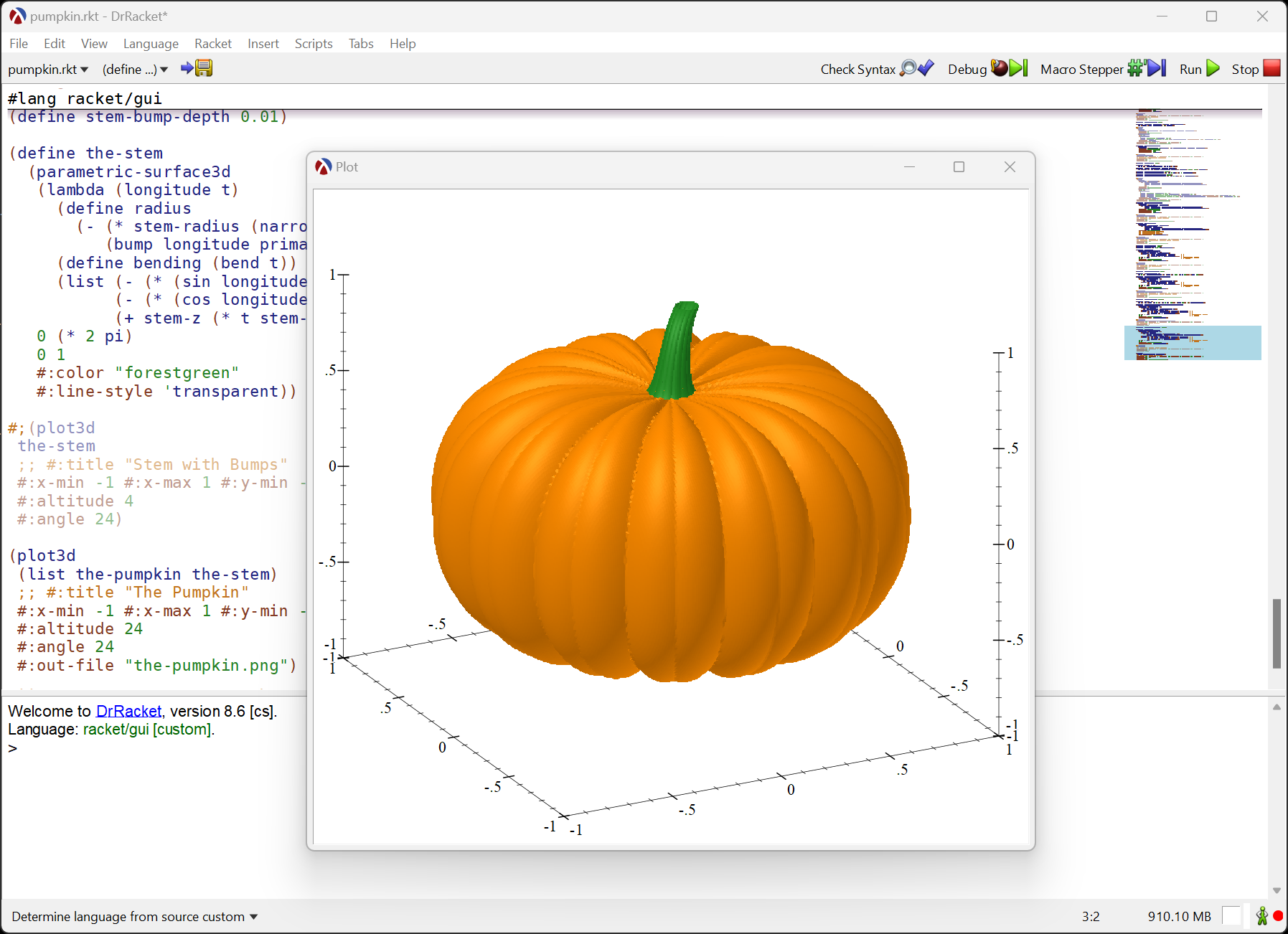
Pumpkin Plot
Inspired by the Digital Arts with MATLAB project, I wanted to check out if the Racket 3D Plot package could be used for a similar purpose, so I decided to plot a pumpkin…
… and here is the result:
This blog post will show a step-by-step guide on how this plot was build, but, before we begin, let’s load the required libraries: we’ll use the plot library for plotting and the pict library for adding some nice labels to the plots:
1 |
(require plot pict) |
There are also a few plot parameters that are useful for this project, these parameters control how the plot looks: how many samples to use for 3D rendering, the width and height of the plot, as well as clearing the labels on the X, Y and Z axes:
1 2 3 4 5 6 7 8 9 10 11 12 13 |
;; open plots in a separate window instead of the REPL (plot-new-window? #f) ;; Number of samples for 3D plots ;; higher values look better, but slower rendering (plot3d-samples 50) ;; The width and height (in pixels) of the plot (plot-width 300) (plot-height 300) ;; Clear the labels of the X, Y and Z axes ;; since they are not meaningfull for a pumpkin (plot-x-label #f) (plot-y-label #f) (plot-z-label #f) |
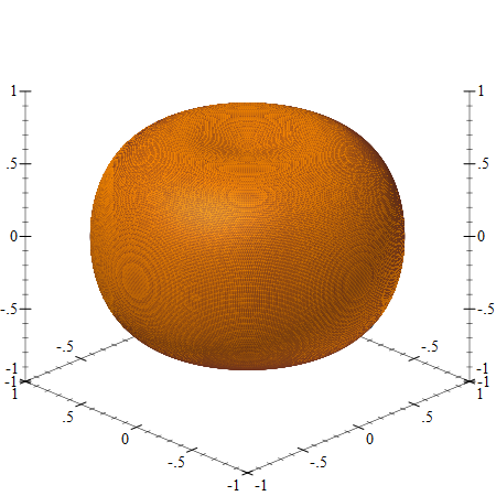
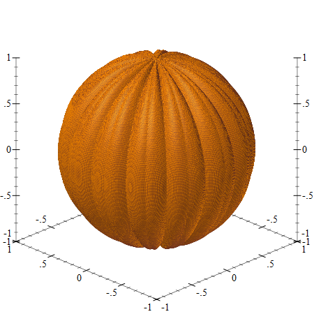
A Sphere
We begin by plotting a sphere, and the simplest way to do that in the racket plot package is to use the polar3d renderer, which plots a function that maps from a Latitude/Longitude pair to a a radius value. Given that we are plotting a sphere, the radius will be a constant:
If you try to display the sphere in the DrRacket REPL, you’ll notice that it does not display anything useful, this is because sphere is just a “renderer”, an object that needs to be passed to one of the plot functions for rendering.
To plot the sphere, we simply pass the sphere to the plot3d function, using (plot3d sphere), and if you run the code in the DrRacket REPL, you can rotate the plot interactively with the mouse:

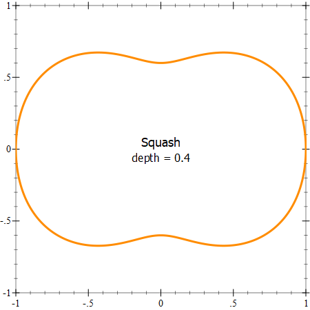
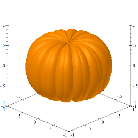
Squashing It
The next step is to “squash” this sphere into a more “pumpkin-like shape” and we’ll use the function sin⁴(x) to reduce the radius of the sphere depending on the “latitude”. Before we build the 3D plot, it might be useful to plot the squashing function separately:
We can plot this function on a 2D plane using the polar renderer, this time we’ll construct and pass the renderer directly to the plot function.
1 2 3 4 5 6 7 8 9 10 11 12 13 14 15 |
(plot (list (polar (lambda (latitude) (- pumpkin-size (squash latitude))) #:width 3 #:color "darkorange") (point-pict #(0 0) (vc-append 2 (text "Squash" 'default 18 0) (text (format "depth = ~a" (~r squash-depth #:precision 2)) 'default 16 0)) #:anchor 'center #:point-sym 'none)) #:x-min -1 #:x-max 1 #:y-min -1 #:y-max 1) |
We can define the “squashed sphere” renderer by simply subtracting the value of the squash function from the radius:
… and we can inspect the result using (plot3d squashed-sphere), and rotate the plot in the DrRacket REPL:
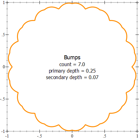
Adding Bumps
A pumpkin should have bumps, and these will be done using a function that modifies the sphere radius along the longitudinal axis. As with the squash function, it is simpler to first visualize the bumps as a 2D plot. We’ll interleave two bumps around the sphere, a “deeper” and a “shallower” one:
1 2 3 4 5 6 7 8 9 10 11 12 13 |
(define num-bumps 7.0) (define (fmod x y) (- x (* (exact-truncate (/ x y)) y))) (define (bump longitude bangle bdepth) (* (expt (- (/ (fmod longitude bangle) bangle) 0.5) 2.0) bdepth)) (define primary-bump-depth 0.25) (define primary-bump-angle (/ (* 2 pi) (* 2 num-bumps))) (define secondary-bump-depth 0.07) (define secondary-bump-angle (/ (* 2 pi) (* 4 num-bumps))) |
And we can plot the bumps outline to adjust the parameters:
1 2 3 4 5 6 7 8 9 10 11 12 13 14 15 16 17 18 19 20 21 |
(plot (list (polar (lambda (longitude) (- pumpkin-size (bump longitude primary-bump-angle primary-bump-depth) (bump longitude secondary-bump-angle secondary-bump-depth) )) #:width 3 #:color "darkorange") (point-pict #(0 0) (vc-append 2 (text "Bumps" 'default 18 0) (text (format "count = ~a" num-bumps) 'default 16 0) (text (format "primary depth = ~a" (~r primary-bump-depth #:precision 2)) 'default 16 0) (text (format "secondary depth = ~a" (~r secondary-bump-depth #:precision 2)) 'default 16 0)) #:anchor 'center #:point-sym 'none)) #:x-min -1 #:x-max 1 #:y-min -1 #:y-max 1) |
As with squashing, we can define a “sphere with bumps” by subtracting the value of the bump function (one for the primary and one for the secondary bump) from the sphere radius, and plotting it using (plot3d
sphere-with-bumps):
The Pumpkin
The squash and bump functions can be combined together, both squasing the sphere and applying bumps to it, making it look like a pumpkin, and plot it using (plot3d the-pumpkin):
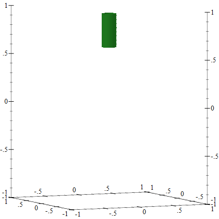
A Cylinder
To make a credible pumpkin, we’ll need a stem, and to plot that, we’ll start with a cylinder. To render a cylinder, we can use the parametric-surface3d renderer — this is a generalization of the polar3d renderer: it still takes a function of two arguments, but allows specifying the range for each of the arguments. In our case, we’ll use the first parameter to specify the “longitude” with a range of 0..2π and another parameter to specify the height of the cylinder, ranging from 0 to 1, this will actually be a percentage of the actual cylinder height, which is defined as stem-length below.
The parametric surface function accepts the two parameters and returns a 3D position, as a list X, Y and Z values. Finally, all the Z values are offset by stem-z, so the cylinder is not drawn at the origin, but at the top of our pumpkin.
The cylinder plotted below is already scaled to match the pumpkin size, but if you find this confusing, it might be worth setting the stem-length to 1, stem-radius to 0.5 and stem-z to 0, so see that this really is a cylinder:
1 2 3 4 5 6 7 8 9 10 11 12 13 14 15 |
(define stem-length 0.35) (define stem-radius 0.1) (define stem-z (- 1.0 squash-depth)) (define cylinder (parametric-surface3d (lambda (longitude t) (define radius stem-radius) (list (* (sin longitude) radius) ; X (* (cos longitude) radius) ; Y (+ stem-z (* t stem-length)))) ; Z 0 (* 2 pi) ; longitude range 0 1 ; t range #:color "forestgreen" #:line-style 'transparent)) |
Here is what it looks like when plotted using (plot3d cylinder), this looks better in the DrRacket REPL, where the plot can be rotated:
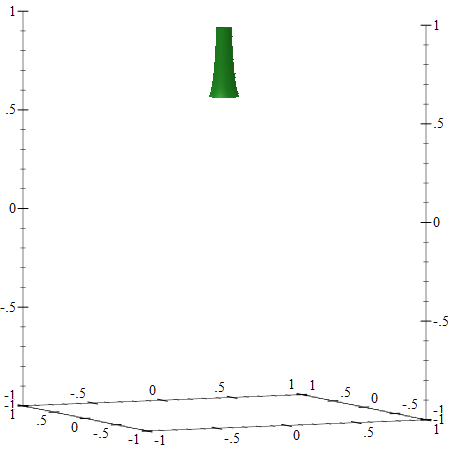
Narrowing
The pumpkin stem needs to narrow as it approaches the top, and we can do that by reducing the cylinder radius based on its height. There are several ways to do that, but I found the function below to work nicely, although it took a few tries to tune the parameters:
Here is the parametric plot which narrows the cylinder, making it resemble a stem, it can be plotted using (plot3d cylinder-with-narrow-top):
1 2 3 4 5 6 7 8 9 10 11 12 |
(define cylinder-with-narrow-top (parametric-surface3d (lambda (longitude t) (define radius (* stem-radius (narrow-stem t))) (list (* (sin longitude) radius) ; X (* (cos longitude) radius) ; Y (+ stem-z (* t stem-length)))) ; Z 0 (* 2 pi) ; longitude range 0 1 ; t range #:color "forestgreen" #:line-style 'transparent)) |
Bending
The stem on a pumpkin is also bent to one side, so we’ll need to bend the cylinder by adjusting the X, Y coordinates of the parametric function. As with narrowing, there are several functions that can be used, but I found the one below, based on logarithms to produce nice results:
We can apply only the bending to the cylinder, to see how it looks, note that we adjust both the X, and Y arguments by the same value, but this is not necessary:
1 2 3 4 5 6 7 8 9 10 11 12 |
(define cylinder-with-bending (parametric-surface3d (lambda (longitude t) (define radius stem-radius) (define bending (bend t)) (list (- (* (sin longitude) radius) bending) ; X (- (* (cos longitude) radius) bending) ; Y (+ stem-z (* t stem-length)))) ; Z 0 (* 2 pi) ; longitude range 0 1 ; t range #:color "forestgreen" #:line-style 'transparent)) |
Here is the output from (plot3d cylinder-with-bending):
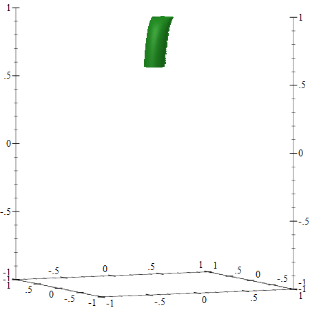
The Stem
To build the actual stem, we’ll start with the cylinder, then we’ll apply the narrowing and bending to it. To make it more realistic, we can also add bumps to it, using the same bump function we used for the pumpkin, the bump value is applied to the stem radius after narrowing it:
1 2 3 4 5 6 7 8 9 10 11 12 13 14 15 16 |
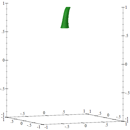
(define stem-bump-depth 0.01) (define the-stem (parametric-surface3d (lambda (longitude t) (define radius (- (* stem-radius (narrow-stem t)) (bump longitude primary-bump-angle stem-bump-depth))) (define bending (bend t)) (list (- (* (sin longitude) radius) bending) ; X (- (* (cos longitude) radius) bending) ; Y (+ stem-z (* t stem-length)))) ; Z 0 (* 2 pi) ; longitude range 0 1 ; t range #:color "forestgreen" #:line-style 'transparent)) |
Here is the output from (plot3d cylinder-with-bending):
Everything Together
To produce the final pumpkin, we can plot the pumpkin and stem renderers on a single canvas by passing both of them to the plot3d command. The plot3d accepts not only a single renderer but also a list (and a list of lists) of renders, making it easy to combine different elements to be plotted:
1 |
(plot3d (list the-pumpkin the-stem)) |
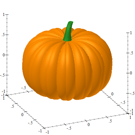
In an interactive DrRacket REPL window, the plot can be rotated using the mouse. Also, the plot3d-samples controls the number of samples used to construct the plot and a low value of 50 will produce a plot where individual faces are noticeable, a higher value (the plot above is rendered using 200 samples) will produce nicer results, but rendering will be slower. Higher sampling values can be used for plots that are saved to image files, for example:
1 2 |
(parameterize ([plot3d-samples 200]) (plot3d-file (list the-pumpkin the-stem) "the-pumpkin.png")) |