A Racket Array Tutorial
If you are unfamiliar with NumPy or Matlab, Racket’s arrays can look strange and unusual, and we’ll try to figure out some use cases for them in this tutorial.
If you are familiar with vector data types, individual element access is important, with program code just iterating over the individual elements of the array to implement data processing. For math/array objects, individual element access is both complicated and inefficient, as the library is designed for operations on entire arrays, but using whole-array, or “lifted” operations requires a change in the way we think about the program code.
To make this tutorial more concrete, we’ll look at a hypothetical "data modeling" task, and see how we can use arrays to model a process as well as data collected from experiments.
Before we begin, the examples below use a few racket libraries which need to be required, so make sure you start your program with the following prelude:
1 2 3 4 5 |
#lang racket (require math/array math/distributions math/statistics plot) |
The Process
Suppose we want to model how errors affect measurements for some real-world process and how we can reconstruct the process function from observations. The process we’ll try to “model” will be defined by the following power function, where the scale, 1.5, and exponent, 3.5 are chosen arbitrarily — we’ll try to rediscover these parameters from observations.
We can plot this function to see how it looks on a graph, and, for power functions it is more interesting to plot them on log-log plots, that is, on plots where axes change logarithmically instead of linearily. The racket plot package supports logarithmic plots directly and, to show it, we’ll define a renderer for this function:
Renderers are not plotted directly, they are an object, or, in our case, list of objects, that can be passed to the plot function. We can plot the function on both a linear and log-log grid by controlling the plot-x-transform and plot-y-transform parameters for the plot:
1 2 3 4 5 6 7 |
(list (parameterize ([plot-title "Linear Grid"]) (plot renderers0)) (parameterize ([plot-title "Log-Log Grid"] [plot-x-transform log-transform] [plot-y-transform log-transform]) (plot renderers0))) |
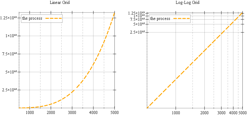
Both these plots show the same function, and, on the linear scale plot, the function shows up as expected for an exponential function. The log-log plot however, shows a straight line — which is also expected, if you are familiar with logarithmic scale plots. If you are not, the function shows up as a line, because the plot package takes the logarithm of our process function and this becomes a line with the slope being 3.5 and intercept being log(1.5):
y = log(f(x)) = log(1.5 * x³͘͘͘ ⁵) = log(1.5) + 3.5 * log(x)To model the data collection from experiments, for our process, we will need to generate some X values for which we take “measurements” and some Y values, which are the actual measurements. For X values, we’ll use evenly spaced numbers between a “low” and “high” end, and, to generate these we’ll need a function called linspace.
The Linspace Function
linspace is a function that constructs a one-dimensional array of evenly spaced numbers over a specified interval. NumpPy has this function built-in, but it is not available in Racket’s math/array library. Fortunately, the implementation is simple, and we’ll have the first oportunity to look at arrays in Racket.
We’ll start by implementing a linspace variant which builds a vector, NOT an array. The function takes as arguments start, stop and num (number of elements) and uses build-vector to produce the result:
Here is how the linspace/as-vector function works:
1 2 |
> (linspace/as-vector 500 5000 10 #t) '#(500 950 1400 1850 2300 2750 3200 3650 4100 4550 5000) |
The linspace variant which builds arrays, is almost identical, but uses build-array instead of build-vector:
There are, however some other differences between linspace/as-array and linspace/as-vector:
- the shape for the array, which for
linspace/as-vectoris just a number, becomes a vector containing one value inlinspace/as-array— this is because arrays can have multiple dimensions and each dimension can have a different number of elements. In our case, however, the resulting array has just one dimension. - the function passed to
build-arrayis slightly different from the one passed tobuild-vector: the build vector variant, receives an index which becomes the element in the vector; the array variant also receives an index, but, since arrays can be multi-dimensional, this index is now a vector of values representing the index on each “axis” or “dimension” of the array. In our case, the index contains one element, since the array has just one dimension.
Here is how the linspace/as-array function works. Notice that the output is different from the linspace/as-vector variant, the result is now an array of one dimension:
1 2 |
> (linspace/as-array 500 5000 10 #t) (array #[500 950 1400 1850 2300 2750 3200 3650 4100 4550 5000]) |
Finally, let’s look at an implementation of linspace which uses array operations. In this implementation, the expression which generates the actual values, (+ start (* span step x)), is “lifted” to work on arrays:
- we start by generating an “index array” of the required shape — this is is an array where each element is the corresponding index, to its location:
(index-array #(4)) => (array #[0 1 2 3]) - next, we create array based versions of the
start,spanandstepscalars — perhaps surprisingly, arrays can have zero dimensions, in which case they hold a single value. - finally, we create the result by applying the linspace “formula”
(+ start (* span step x))to our arrays usingarray+andarray*operations instead of using+and*:
1 2 3 4 5 6 7 8 9 10 |
(define (linspace start stop [num 50] [endpoint? #t]) (define shape (vector (if endpoint? (add1 num) num))) (define indexes (index-array shape)) (define a-start (array start)) (define a-span (array (- stop start))) (define a-step (array (/ 1 num))) (array+ a-start (array* a-span (array* a-step indexes)))) |
You might be wondering how is it possible for an expression such as (array* a-step indexes) to work, since a-step is an array of zero dimensions with one element, while indexes is an array of one dimension of num elements. In our case, it multiplies the value of a-step with each value from the indexes array. This is called broadcasting and the description for how it works is found in the broadcasting section of the math/array library documentation.
And, of course, we can verify that this version of linspace also works as expected:
1 2 |
> (linspace 500 5000 10 #t) (array #[500 950 1400 1850 2300 2750 3200 3650 4100 4550 5000]) |
The Observatios
We can use linspace to generate an array of X values for which we will “measure” our process function as follows:
1 |
(define xs (linspace 500 5000 20 #t)) |
There are several options for generating the Y values which correspond to each value from the xs array. The first option is to use array-map:
1 |
(define ys (array-map the-process xs)) |
Another option is to use lifted array operations and express the process in terms of these. There is no array-expt function in the array library, but we can easily define it. In this case the “process” expression is more visible when the ys array is generated:
The ys array contains exact values for our “process” function, to model real world data collection, we can add some errors to our observations. We’ll first build an array of error values drawn from a normal distribution and add the errors to the ys array. We build our errors array with the same shape as the ys array:
Finally, we can “add” these errors to our ys array. There are several ways to add errors to observations, in our case, we’ll multiply each Y value with the error, since simply using addition will add small values to the large exponential values produced by our process function, and this will not produce visibly different measurements. Of course, you can model any kind of errors, including no errors at all — but this method produces nice looking plots…
1 |
(define ys-observations (array* ys (array+ (array 1) errors))) |
Plotting the observations
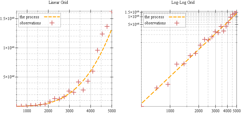
We can plot the observations as individual data points using points plot renderer, however, this renderer expects a single sequence of points with the X and Y “packed” in a vector, while we have separate xs and ys arrays. However, it is easy to convert these two arrays into one using array-map:
(define observations
(array-map (lambda (x y) (vector x y)) xs ys-observations))We can add the observations to our renderers:
… and plot them in both linear and log-log grids. Note how in both cases, the observations follow the “process” line, although with some errors:
1 2 3 4 5 6 7 |
(list (parameterize ([plot-title "Linear Grid"]) (plot-pict renderers1)) (parameterize ([plot-title "Log-Log Grid"] [plot-x-transform log-transform] [plot-y-transform log-transform]) (plot-pict renderers1))) |
Linear Regression
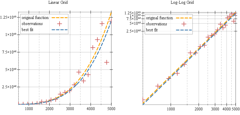
We started with a known “process” and we generated some sample observations which contained some errors. We can now try the reverse operation, where we attempt to determine the original process from our sample observations — this is the method that would be applied in the real world, where some measurements would be obtained thrhough some experiment and we would attempt to reconstruct the original process function from these.
The insight for doing this relies on the observation that, on the log-log plot, all measurements are on a straight line, and we can determine the slope and intercept of this line using Simple Linear Regression. The details of this process are beyond this blog post, but, in short, it allows us to determine the line that best approximates a set of observations using their average, standard deviation and correlation.
Racket has no function to calculate the linear regression of a set of observations, but all the basic ingredients are available in the math/statistics library. First, the mean and standard deviation of a data set can be constructed using a statistics object using update-statistics. Here is how we “reduce” a one dimensional array to a single statistics object, using the array-all-fold function.
There is a correlation function in the Racket statistics library, however that one works on sequences instead of arrays. Here is how to write an array-correlation function which determines the correlation between two arrays:
1 2 |
(define (array-correlation a b) (correlation (in-array a) (in-array b))) |
With these two operations defined for arrays, we can define a simple-linear-regression function as shown below. The function returns two values, a slope and an intercept:
1 2 3 4 5 6 7 |
(define (simple-linear-regression xs ys) (let ((x-stats (array-statistics xs)) (y-stats (array-statistics ys)) (r (array-correlation xs ys))) (let* ((slope (* r (/ (statistics-stddev y-stats) (statistics-stddev x-stats)))) (intercept (- (statistics-mean y-stats) (* slope (statistics-mean x-stats))))) (values slope intercept)))) |
We cannot apply simple-linear-regression directly to our xs and ys-observations arrays, since they are observations for a power function, this function only appears linear in log-log space. Instead we need to do the regression on the logarithms of these values, which is what the plot library does when it transforms the data for plotting. We can write another short helper function to take the logarithm of an array like so:
… and with this defined, we can obtain the slope and intercept values for the line that best matches our observations:
1 2 |
(define-values (slope intercept) (simple-linear-regression (array-log xs) (array-log ys-observations))) |
If you inspect the slope and intercept, you’ll notice that slope matches the original slope of 3.5 closely, but the intercept value does not match our scale value of 1.5 in the original function. This is because, when converting to log-log space, the “intercept” is actually the logarithm of this scale value, so we need to use exp on the intercept value:
y = log(f(x)) = log(1.5 * x³͘͘͘ ⁵) = log(1.5) + 3.5 * log(x)The “best fit” function for our data set can be defined as:
Finally, we can add our “best fit” line to the plot to see how it matches up:
… and plot them in both linear and log-log grids:
1 2 3 4 5 6 7 |
(list (parameterize ([plot-title "Linear Grid"]) (plot-pict renderers2)) (parameterize ([plot-title "Log-Log Grid"] [plot-x-transform log-transform] [plot-y-transform log-transform]) (plot-pict renderers2))) |
A few notes if you try to run these examples yourself:
- the values for the observations, and the slope and intercept for the best fit will be different every time you try to run the program. This is because the errors added to the
ysarray will be different every time the program is run. - the best fit parameters, slope and intercept, will be poor fit in the examples above, this is because we generate a small number of samples for our observations and the error is large. This is done so the plot is not overly cluttered, but it does produce poor regression results. Regression values can be improved by generating larger number of samples for the
xsarray, for example 100 samples seems to work well.
Final Thoughts
The math/array Racket library allows working with multi-dimensional arrays without having to work with iteration, either as a for loop or as a map operation. It is a common way of working in signal processing applications as supported by Matlab and Numpy, but it is not common to see arrays in Racket code, perhaps because Racket is not used for such applications. math/array is stil useful as a library, and enables some programming techniques that would be more cumbersome otherwise.